- Author Jason Gerald gerald@how-what-advice.com.
- Public 2024-01-19 22:11.
- Last modified 2025-01-23 12:04.
This article will guide you to enter data into a pivot table in Microsoft Excel. This guide can be followed on Windows and Mac versions of Microsoft Excel.
Step

Step 1. Double-click the Excel document containing the pivot table
The document will open.

Step 2. Click the tab containing the data you want to enter (eg Sheet 2) at the bottom of the Excel window

Step 3. Add or change the data you want to insert into the pivot table next to or below the existing data
- For example, if you already have data in cells A1 through E10, you can enter the data in column F or in row 11.
- If you only want to change the data that appears in the pivot table, change that data in the active worksheet.

Step 4. Return to the tab containing the pivot table by clicking on the tab name
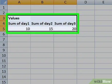
Step 5. Click the pivot table to select it
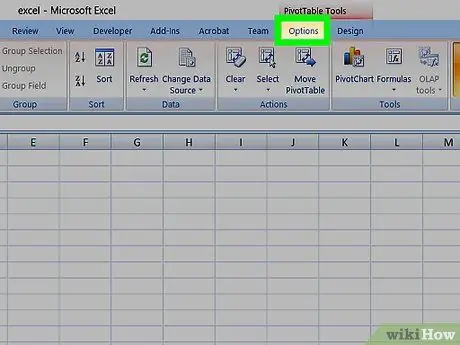
Step 6. Click the Analyze button in the middle of the green ribbon in the Excel window
You will see a new toolbar below the ribbon.
If you are using a Mac, click the tab PivotTable Analyze.
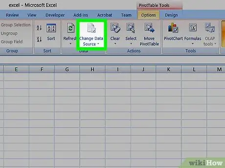
Step 7. Click the Change Data Source button in the "Data" section of the "Analyze" toolbar
You will see a drop-down menu.
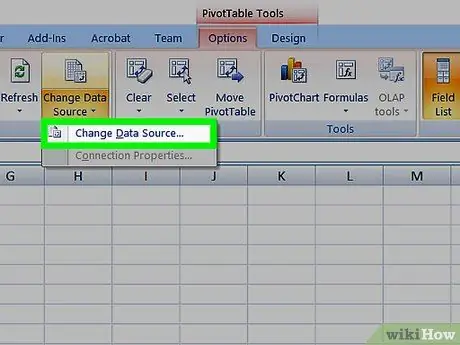
Step 8. From the menu, click Change Data Source…
A new window will open.

Step 9. Select your data
Click and drag the cursor from the top left cell to the bottom left. Cells containing the data you have entered will be selected as well.
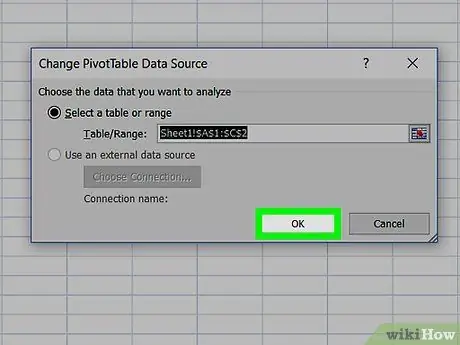
Step 10. Click OK at the bottom of the window


