- Author Jason Gerald gerald@how-what-advice.com.
- Public 2023-12-16 10:50.
- Last modified 2025-01-23 12:04.
If your Excel spreadsheet is filled with a lot of blank rows, manually deleting all of them can be tedious. It's easy enough for you to delete a single line, but deleting a lot of blank lines might be quite a burden for you. Fortunately, there are several tools you can use to make the process of removing blank lines easier.
Step
Method 1 of 2: Deleting One Line
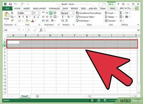
Step 1. Find the row you want to delete
If you only have a line or two that need to be deleted, you can do this quickly with your mouse.
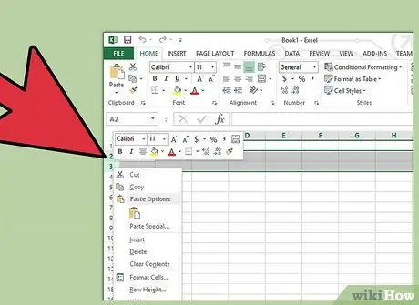
Step 2. Right click on the row number you want to delete
The start to the end of the line will be selected when you right click on the line number.
If there are several blank rows next to each other, click and hold on the number of the first blank row, then drag the mouse until you reach the last row you want to delete. Right click on the selected region
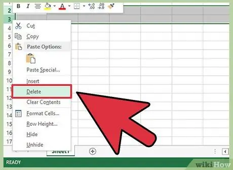
Step 3. Select "Delete"
The blank row will be deleted, and the rows below it will move up to fill the blank space. The numbers of all rows below will be readjusted.
Method 2 of 2: Deleting Multiple Rows
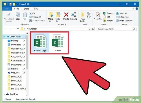
Step 1. Back up the worksheet
Whenever you drastically change a worksheet, it's always a good idea to back up the worksheet first so you can restore the worksheet next time. You can do this by simply copying and pasting the worksheets into the same directory for a quick backup.
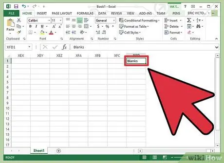
Step 2. Add a column far at the far right of the worksheet labeled "Blank"
This method works by quickly filtering out blank rows so you can be sure that you don't accidentally delete rows that contain unseen data. This method is very useful, especially for large worksheets.
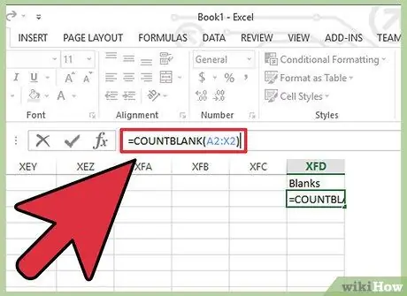
Step 3. Add the blank row counter formula to the first cell in the new column
Enter the formula =COUNTBLANK(A2:X2). Replace X2 with the last column in the worksheet that is in the position before the "Blank" column. If the worksheet does not start from column A, replace A2 with the starting column of the worksheet. Make sure that the row numbers match the initial data on the worksheet.
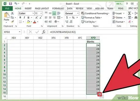
Step 4. Apply the formula to the entire column
Click and drag the small square in the corner of the cell to apply the formula to all "Blank" columns, or double-click to apply it automatically. Each cell in the column will be filled with the number of blank cells in each row.
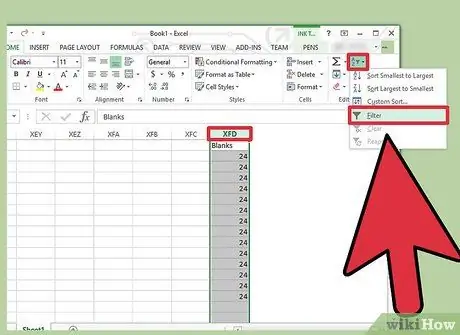
Step 5. Select the entire "Blank" column, then click "Sort and Filter" → "Filter"
You will see a drop-down arrow in the head cell section.
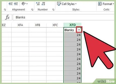
Step 6. Click the drop down arrow to open the Filter menu
The menu allows you to choose how to filter the displayed data.
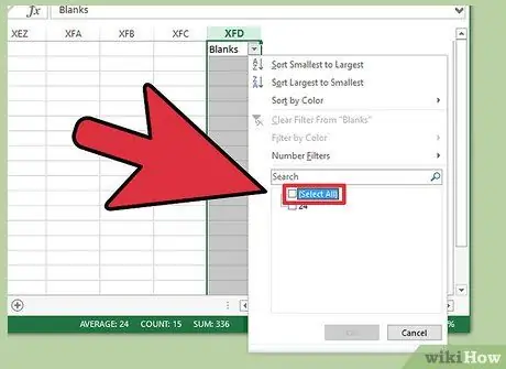
Step 7. Uncheck the "Select All" box
That way, all data with different values will not be selected, and the data will be selected automatically.
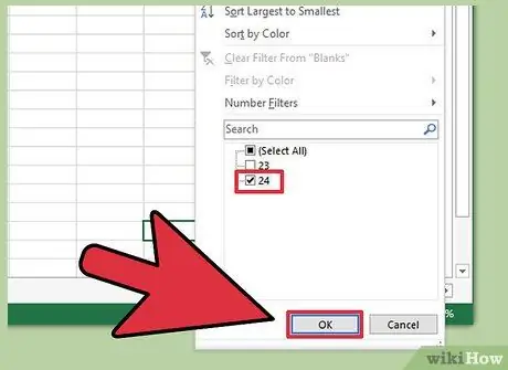
Step 8. Check the boxes that have values that correspond to the number of columns in your worksheet
Click "OK". By checking the box, the rows that are displayed are only rows with blank cells in each cell. This way, you can be sure that you won't delete rows that have useful data at the same time as empty cells.
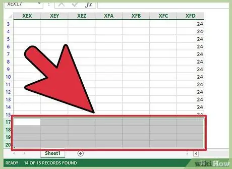
Step 9. Select all blank rows
You should only see rows with blank cells. Select all rows to delete.
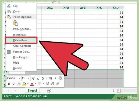
Step 10. Delete the selected blank rows
After selecting all blank rows, right click on all selected rows, then select "Delete". Blank rows will be deleted from within the worksheet.
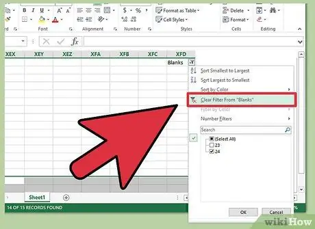
Step 11. Turn off the filter
Click the Filter button on the "Blank" row, then select "Clear Filter". Your worksheet will return to the way it was before, and all blank rows will disappear. Other data will remain in the worksheet.


