How to Create a Simple Check Register in Excel (with Pictures)

2024 Author: Jason Gerald | [email protected]. Last modified: 2023-12-16 10:50

Check account activity is easier to record using check registers created from Microsoft Excel. You can set up check registers to categorize expenses so you can track any money spent. You can create a formula to find out the balance of money in the account. Besides being useful, by creating a check register in Excel you can also know the basics of Excel.

Step

Part 1 of 5: Creating Columns in Excel

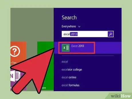
Step 1. Get to know Excel

Excel is a spreadsheet software used to manage data and perform calculations with formulas. Excel spreadsheets are organized by columns and rows.

The desktop version of Excel can be installed on a PC or Mac. There are also free online apps for your computer, tablet or phone. The functionality of each version is only slightly different.
Excel has been around for a long time, and there's always a new version every year. The way each version works is only slightly different.
In Excel, rows are horizontal and sorted by number. Columns are vertical and sorted by letter. The squares where rows and columns meet are called cells. Cells are named after rows and columns. The cell in the fifth row in column D is named D5 (column D, row 5).
Know the difference between a worksheet and a workbook. A worksheet is an Excel file that contains one or more spreadsheets. Each spreadsheet is in separate tabs within the workbook. Workbooks generally have three tabs, but can be added if necessary.
You can simply use one tab to create a basic check register.
You will use the two tabs to create a load category function in the check register.

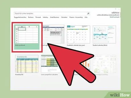
Create a Simple Checkbook Register With Microsoft Excel Step 2

Step 2. Open a blank spreadsheet

How to open a spreadsheet depends on the operating system and the type of computer you are using.

For PCs running an operating system under Windows 7, click the Start menu in the lower-left corner of the desktop. From the menu that appears, click Programs. From the menu that appears next, click Microsoft Office, then click Microsoft Office Excel. At this point a blank spreadsheet appears on your desktop.
For PCs on Windows 7 or later, click the Windows icon in the lower-left corner of the screen, then click the Microsoft Excel tile to open Excel. There will be a page showing the new files on the left and the new document template options on the right. Click the first template option, Blank Workbook to open a new spreadsheet.
To open Excel on the Mac, click Excel in the dock. Click "File" in the menu bar. Click "Open" then click "New". You will be taken to a new blank spreadsheet.

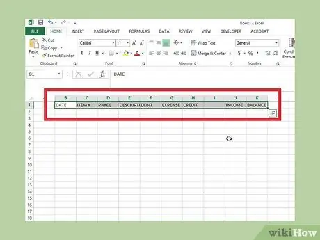
Create a Simple Checkbook Register With Microsoft Excel Step 3

Step 3. Create column labels

Use the label that is usually found in the register check book. Create columns for date, no. check, payee, and description or memo. Then create columns for debits (i.e. payments or withdrawals), credits (i.e. deposits) and forward balances.

Enter "DATE" in cell B1 (column B, row 1). The transaction date is entered here.
Move one cell to the right, cell C1 (column C, row 1). Type "ITEM #". The check number or transaction type is entered here, such as "ATM" or "deposit".
Move one cell to the right, cell D1 (column D, row 1). Type in "PAYEE". This is the name of the recipient of the check or payee.
Move one cell to the right, cell E1 (column E, row 1). Type "DESCRIPTION". Details about the transaction are entered here.
Move one cell to the right, cell F1 (column F, row 1). Type "DEBIT". The money that goes out of the account (outflow) is recorded here.
Move one cell to the right, cell G1 (column G, row 1). Type "EXPENSE CATEGORY". Leave this blank first. These column options will be created in a later step.
Move one cell to the right, cell H1 (column H, row 1). Type "CREDIT". Money that goes into the account (inflow) is recorded here.
Move one cell to the right, cell J1 (column J, row 1). Type "INCOME CATEGORY". These column options will also be created in a later step.
Move one cell to the right, cell K1 (column K, row 1). Type "BALANCE". This is the amount in the account after all transactions have been recorded.

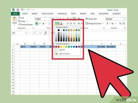
Create a Simple Checkbook Register With Microsoft Excel Step 4

Step 4. Format the column labels

Add formatting to the label column in bold font and give the register label rows a different background color for easy reading. First, select the range of cells you want to format, then select a format option.

Look for the format options in the "HOME" tab of the toolbar ribbon. This "HOME" tab is already open when you open a new workbook.
Select cell B1 (DATE) then drag the cursor on all labels until cell K1 (BALANCE).
In the top left corner of the toolbar, click "B" to select a bold format.
Click the paint bucket icon to view the background color palette to change the background color.

Create a Simple Checkbook Register With Microsoft Excel Step 5

Step 5. Resize multiple columns

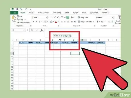
Usually the column size is too small to store the data you entered. For example, the “PAYEE” and “DESCRIPTION” fields can hold long names or long memos. Column A only serves as a separator, so its size is very narrow.

Click the column header A to select the entire column. In the top right corner of the toolbar on the "HOME" ribbon, click the "FORMAT" button. From the drop-down menu, click "Column Width", enter 2 then click OK. Column A will be very narrow.
Expand column D, "PAYEE". Click the header section in column D to select that column. Hover over the border of columns D and E. The cursor will change to a resize cursor, with a shape like a plus sign with an arrow pointing. Once this cursor is visible, left click and drag the mouse to the right to make the column as wide as you want.
Repeat the same procedure to expand column E, "DESCRIPTION".

Create a Simple Checkbook Register With Microsoft Excel Step 6

Step 6. Center the register label

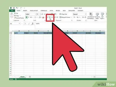
Select the entire first row. Left-click the number one on the left border of the page. On the top left side of the toolbar on the "HOME" ribbon, click the center align button. All data in the selected cells will be centered. The column labels in each cell are now centered.

Part 2 of 5: Formatting Cells

Create a Simple Checkbook Register With Microsoft Excel Step 7

Step 1. Enter Some data

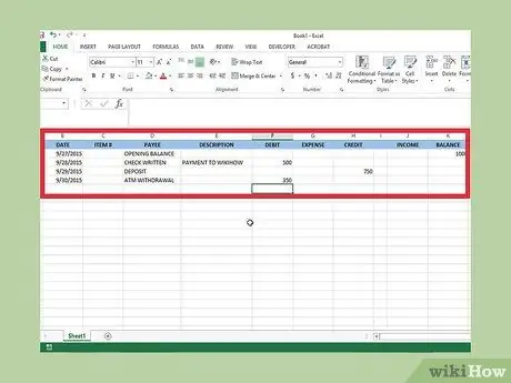
To see the format changes made, enter four rows of data into the cells. Start with the starting balance, then enter the other three transactions.

Add the date for the opening balance into cell B2, for example 9/27/15. In the "PAYEE" column in cell D2, type "Opening Balance". In the "BALANCE" column in cell K2, enter the amount of money in your account according to the date in cell B2.
Add three more transactions. Combine debit transactions (such as check payments or ATM withdrawals) and credit transactions (such as deposits).
Notice the inconsistent formatting of each number in the cell. The date column format might change to "2015/09/27" or "27-Sept". The dollar amount column may display the wrong number of decimal places. Format it so that everything is clean.

Create a Simple Checkbook Register With Microsoft Excel Step 8

Step 2. Format the date

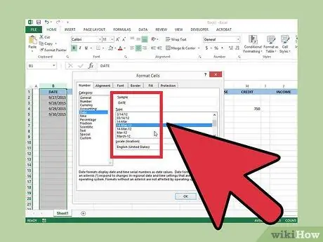
Make sure this column displays consistent dates. There are many options for formatting dates in Excel. Choose which one you want.

Click the header in column B, which is "DATE". All columns will be selected.
Right-click on the column and select Format Cells. The Format Cells window will appear.
Select the "Numbers" tab. Select "Date" in "Category". Select the date format you want and click OK in the lower right corner of the window.
While the column is still selected, center the data in these cells by clicking the center-align icon in the top-left corner of the toolbar, in the "HOME" ribbon.

Create a Simple Checkbook Register With Microsoft Excel Step 9

Step 3. Format Column "ITEM #"

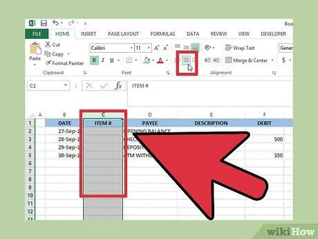
The data in this column must be centered. Highlight the entire column of C by clicking on the column header. Click the center align icon. Pay attention to the data that has been entered in this column. The writing must be centered.

Check the format of columns D and E, "PAYEE" and "DESCRIPTION". Excel usually formats cells so that the data is left aligned. This format will be suitable for this column. Double check the column size. There is now some data in these cells, so adjust the column width to make the column wider or narrower, as needed

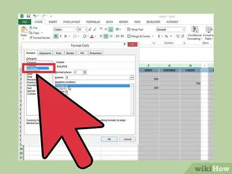
Create a Simple Checkbook Register With Microsoft Excel Step 10

Step 4. Format the currency in columns F, H and K, or "DEBIT," "CREDIT" and "BALANCE FORWARD"

Currency uses two-digit decimals. There is an option to display dollar signs. The debit number can also be made red if you wish.

Select column F. Right-click in column F and select Format Cells. The Format Cells window will appear. On the "Number" tab, select "Accounting". Select "2" in the "Decimal places" option. Select the dollar sign in "Symbol".
Repeat the above steps for columns H and K.
To make the debit number look red, click the header in column F to select the entire column. Right-click the column and select Format Cells. Select the Font tab when the Format Cells window appears. On this tab, click the drop-down next to the Color option. From the palette, click the red color.

Part 3 of 5: Creating Formulas

Create a Simple Checkbook Register With Microsoft Excel Step 11

Step 1. Create a formula to calculate the current balance

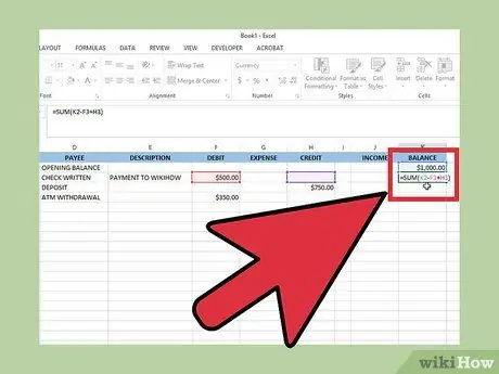
Enter the mathematical operation formula to calculate the current balance into column K. You don't need the formula in cell K2. Your starting balance is entered here.

Click cell K3. Click the formula bar at the top of the spreadsheet. Type in the formula to perform the calculation. Enter =SUM(K2-F3+H3). This formula tells the spreadsheet to take the opening balance (cell K2), subtract debits if any (cell F3), and add credits if any (cell H3).
If the opening balance is $200, and your first entry is a check for $35, record $35 as a debit in cell F3. The formula you entered in cell H3 takes the initial balance and subtracts the debit so that the balance remains at $165.

Create a Simple Checkbook Register With Microsoft Excel Step 12

Step 2. Copy the formula

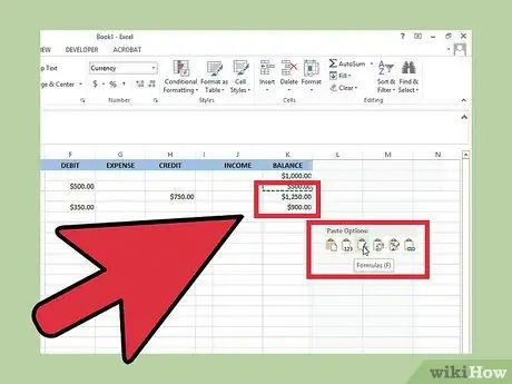
Select cell K3. Right click and select Copy. Select cells K4 and K5, then right-click and select Paste. Now the formula is copied to these cells. Now the current balance has been calculated in column K for all the data rows that have been entered.

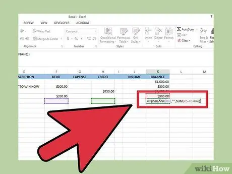
Create a Simple Checkbook Register With Microsoft Excel Step 13

Step 3. Create a conditional formula to clear the current balance column

You can copy the above formula to cell K6. However, since you have not entered any data, the current balance from cell K5 will also appear in cell K6. To clear this up, create a conditional formula that will empty the cell if no transactions are entered, but will display the balance if there is one.

In cell K6, enter the formula =IF(ISBLANK(B6), "", SUM(K5-F6+H6)). This will tell Excel that if cell B6 in the "DATE" column is empty, cell H6 must be blank, but if cell B6 is not empty, the balance should be calculated

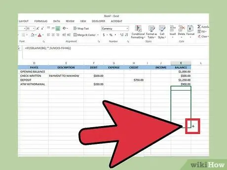
Create a Simple Checkbook Register With Microsoft Excel Step 14

Step 4. Expand the formula with AutoFill

The AutoFill feature fills the formula of adjacent cells so there is no need to enter the "BALANCE" formula repeatedly.

Look for the AutoFill lever in the active cell. Look at the small dark rectangle in the lower right corner of the active cell. Hover the cursor until it changes to an AutoFill cursor, which looks like a thin plus.
Click on cell K6. Hover over the AutoFill lever and the cursor will change to a thin plus sign. Left click and hold the AutoFill lever. Drag the cursor to cell K100 (column K, row 100).
The formula is now copied to all cells column K through row 100. The row and column numbers in each cell are automatically adjusted so that the formula can calculate correctly.

Part 4 of 5: Adding Categories

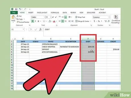
Create a Simple Checkbook Register With Microsoft Excel Step 15

Step 1. Create a transaction category

Transaction categories are useful for tracking cash outflows and income types. Categories can relate to income taxes, such as property taxes or charitable contributions. Categories can also be used to create charts that easily visualize an account's financial activity.

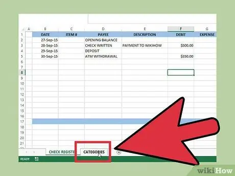
Create a Simple Checkbook Register With Microsoft Excel Step 16

Step 2. Create the "Categories" tab

This tab is used to store all potential categories of income and expense register checks. Rename one of the tabs in the "Categories" workbook. Double-click an existing tab title so that it highlights the name. The name will change to "Sheet2" or "Sheet3". When the sheet name is highlighted, type a new name for the tab, such as "Categories".

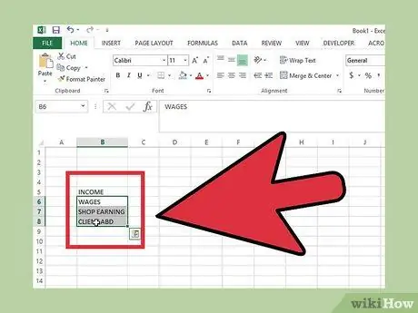
In cell B4, type "Categories". Format the cells to be bold and center them

Create a Simple Checkbook Register With Microsoft Excel Step 17

Step 3. Create income categories

Type "*** Income ***" in cell B5. All categories of income that you have or can benefit from in the future are included here. Enter all your income categories starting from cell B6 and working your way down.

The most common income category is "Wages" (wages). Break down the different wage categories if there is more than one job.
Your financial situation is a determining factor for other income categories. Create a "Dividend" category if you own shares. Also create child support categories if applicable. Other categories such as “Interest Income,” “Gifts”, and “Miscellaneous”.

Create a Simple Checkbook Register With Microsoft Excel Step 18

Step 4. Create load categories

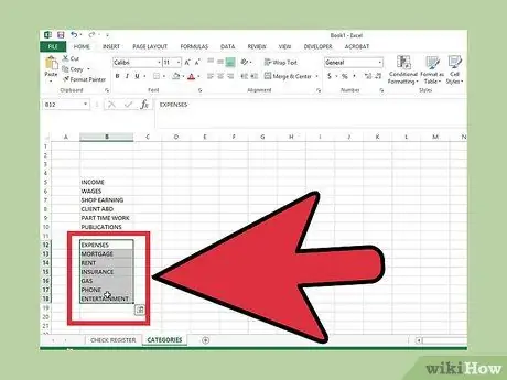
Clear the cells in the last income category. Move one cell down and then type "*** Expenses ***". All load categories are in this section.

The number of load categories is tailored to your circumstances, including “Mortgage,” “Rent,” “Insurance,” “Car Payment,” “Gas,” “Electricity,” “Phone”, or “Entertainment”

Create a Simple Checkbook Register With Microsoft Excel Step 19

Step 5. Give a name to the range of cells containing the category

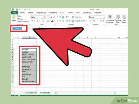
Select cell B5, then highlight from cell B5 to all income and expense categories. Look for the cell name box in the upper-left corner of the window, which is to the left of the formula box. The name of the first cell in the highlighted range will display "B5". Click the cell name box and type "Categories". This is the name of the range of cells that you can use in the check register.

Create a Simple Checkbook Register With Microsoft Excel Step 20

Step 6. Use the expense and income categories in the check register

Go back to the tab you created the check register. Now the “EXPENSE CATEGORY” and “INCOME CATEGORY” columns will be added to a drop-down menu.

Select cell G2 in the register tab check. This is the first cell in the “EXPENSE CATEGORY” column.
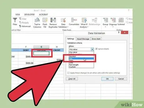
Select the "DATA" ribbon in the toolbar. Click the "Data Validation" button. Select “Data Validation” from the drop-down menu. The “Data Validation” window will open.
On the "Settings" tab of the "Data Validation" window, find the "Allow" drop-down box. Click the down arrow and select "List". Enter "=Categories" under "Source". click OK.
A small arrow will appear next to cell G2. Click this arrow to display a list of categories. Click the category that corresponds to the row transaction.
Copy the formula from cell G2 to cell G100 using AutoFill.
Go to cell J2 to repeat the process in the “INCOME CATEGORY” column.

Part 5 of 5: Protecting the Check Register

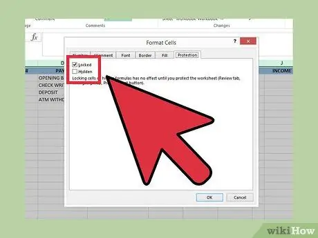
Create a Simple Checkbook Register With Microsoft Excel Step 21

Step 1. Lock formula cells and protect spreadsheet

Protecting the worksheet means you can't overwrite data in locked cells so you don't have to worry about future balance calculations being wrong because of formula errors. You can also add a password to make your check register more protected from other users. Make sure the password is easy to remember, or write it down in a safe place. The worksheet will not be accessible if you forget your password.

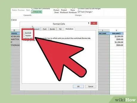
Create a Simple Checkbook Register With Microsoft Excel Step 22

Step 2. Unlock the cell

Once the worksheet is protected, all cells will be locked. Therefore, you must unlock the data cells to be entered, even if the worksheet is protected.

Select cells B2 to J100. These are all cells of all check register columns, except the last column, K, which is the "BALANCE" column. Data must still be entered into these cells even if the worksheet is protected.
In the selected range of cells, right-click. Select Format Cells.
In the Format Cells window, select the Protection tab. Uncheck the “Locked” box then click OK.

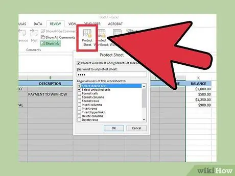
Create a Simple Checkbook Register With Microsoft Excel Step 23

Step 3. Enable Protection on the worksheet

This means that all cells will remain locked, including the cells in column K ("BALANCE") so they cannot be overwritten.

Open the "REVIEW" ribbon in the toolbar. Click “Protect Sheet” to bring up the “Protect Sheet” window.
If you want to protect the worksheet, add the password here. If not, leave it blank.
click OK. Check registers are now unprotected.

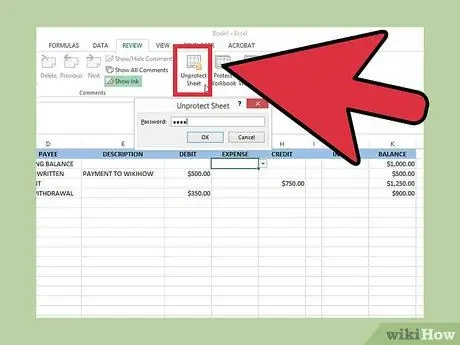
Create a Simple Checkbook Register With Microsoft Excel Step 24

Step 4. Unprotect the worksheet in order to change the locked cells

You can reverse this process later if you want to change the formula in a locked cell. Open the "REVIEW" ribbon in the toolbar. Click "Unprotect Sheet" until the "Unprotect Sheet" window appears. click OK.