- Author Jason Gerald gerald@how-what-advice.com.
- Public 2024-01-19 22:11.
- Last modified 2025-01-23 12:04.
The amortization schedule shows the interest that is applied to a fixed-rate loan and the reduction of the principal loan by repayment. The schedule also shows a detailed schedule of all payments so you can know the amount that goes into the principal loan and what is paid out as interest expense. An amortization schedule is very easy to create with Microsoft Excel. Start with Step 1 to set up an amortization schedule at home without having to pay someone else to do it!
Step
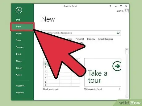
Step 1. Open Microsoft Excel and open a new spreadsheet
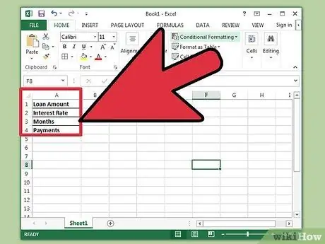
Step 2. Label cells A1 to A4 as follows:
Loan Amount, Interest, Month and Payment.
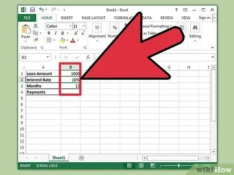
Step 3. Enter the information related to the loan in cells B1 to B3
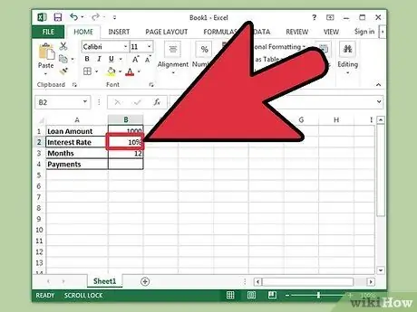
Step 4. Enter the loan interest rate as a percentage
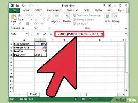
Step 5. Calculate the payment in cell B4 by typing " =ROUND(PMT($B$2/12, $B$3, -$B$1, 0), 2)" into the formula box without quotes and then press Enter
- The dollar sign in the formula is for absolute reference so that the entered formula always looks up the specified cell, even if the formula is copied to any part of the worksheet.
- The interest rate must be divided by 12 because it is an annual interest which is calculated on a monthly basis.
- For example, if your loan is $150,000 at 6 percent interest for 30 years (360 months), the loan repayments are $899.33.
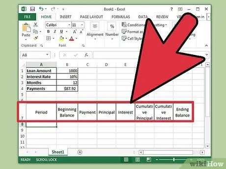
Step 6. Label cells A7 to H7 as follows:
Period, Initial Balance, Payment, Principal Loan, Interest, Cumulative Principal Loan, Cumulative Interest and Ending Balance.
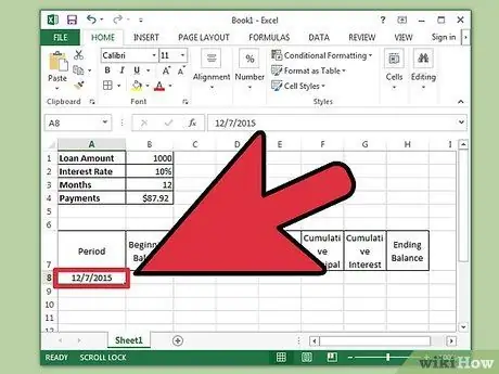
Step 7. Enter values into the Period column
- Enter the month and year of the first loan payment into cell A8. The column must be formatted so that it displays the month and year correctly.
- Select the cell, click and drag down to fill the column up to cell A367. Make sure the Auto Fill Option is set to " Fill Months."
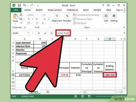
Step 8. Complete the process of entering data in cells B8 to H8
- Enter the opening balance in cell B8.
- Type "=$B$4" in cell C8 then press " Enter."
- In cell E8, create a formula to calculate interest on the beginning balance for the period. The formula is "=ROUND($B8*($B$2/12), 2)". The single dollar sign is used to create a relative reference. The formula will search for the appropriate cell in column B.
- In cell D8, subtract the loan interest amount in cell E8 from the total payment in C8. Use relative references so that these cells can be copied correctly. The formula is " =$C8-$E8."
- In cell H8, create a formula to subtract the portion of the principal loan payment from the beginning balance for the period. The formula is " =$B8-$D8."
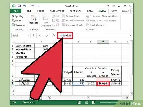
Step 9. Continue the schedule by making the following entries in cells B9 to H9
- Cell B9 must contain a reference relative to the ending balance of the previous period. Type "=$H8" in the cell and then press Enter key. Copy cells C8, D8, and E8 and paste them into C9, D9, and E9. Copy cell H8 then paste into H9. The benefits of relative reference can be felt at this step.
- In cell F9, enter the formula for tabulating the cumulative principal loan paid. The formula is: " =$D9+$F8." Do the same for the cumulative interest cell in G9, namely: " =$E9+$G8."
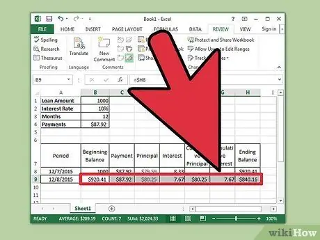
Step 10. Complete the amortization schedule
- Highlight cells B9 to H9, move the cursor over the lower right corner of the selection of cells until a black plus cursor sign appears. Click and drag the selection up to line 367. Release the mouse button.
- Make sure the Auto Fill Option is set to "Copy Cells" and the final balance is $0.00.
Tips
- Now you can scroll through any loan repayment period to see the amount of payments on the principal loan, the amount charged as interest on the loan, and the amount of the principal plus interest paid to date.
- If the final balance is not $0.00, make sure that the formula used relative and absolute references according to the instructions and that the cells have been copied correctly.


